Multidimensional Query System of Equations

Thinking about the high technologies of our modern lives, it is humbling to realize that what we take for granted today is built on top of mathematical and scientific discoveries made thousands of years ago.  For example, around 4000 years ago, the people of Babylon knew how to solve a simple 2X2 system of linear equations with two unknowns. Later on, around 200 BC, the Chinese published the book called “Nine Chapters of the Mathematical Art,” which described the ability to solve a 3X3 System Of equations.  What they were trying to figure out was a way to map out vector spaces, lines, planes, and subspaces.  The understanding of these ideas provided the fundamental basis of how data can be located and retrieved in a multi-dimensional space.

Where Have I Seen This Before?

Let’s take a look at how these ideas have benefited us.  If you have used Excel spreadsheets before, more than likely you would have come across a built-in reporting tool called pivot table.  To illustrate what a pivot table is, imagine that you have a reporting tool which generates a report for you automatically simply by choosing items from a list and dragging and then dropping them into the pivot table.  The list of items are separated into two groups.  The first group is called metrics and the second group is called dimensions.  The metrics are items on the list that can be measured using arithmetic operations such as adding, subtracting and so on, and the dimensions are items that describe the metrics.

Example

Let’s take a look at an example to illustrate these two groups.  A company has the following list items: Sales, Date, Geography and Products.  The metric in this list is ‘Sales’.  If we drag the Sales item to the pivot table and suppose the amount is $1,000,000, this is not very helpful because the sales amount does not give us any information about what that sales amount is referring to.  Therefore, we need describing items to give context to this sales amount.  The contextual items in our example list are: Date, Store and Product.  We call the grouping that contains these types of items ‘Dimensions’.

If you want to know how much sales was generated in Jan 2016, Northern Store and widget X, you would do the following:

1. Drag sales to the center of the pivot table.
2. Drag Date to column axis filtered by ‘Jan 2016’
3. Drag Store next to the Date in the column axis filtered by ‘Store A’
4. Drag Product next the Store in the column axis filtered by ‘Widget Y’

Your result should looking something like this:

Date                    Store                   Product               Sales

Jan 2016            Store A               Widget Y             $100,000

Now that we have a general idea of what a pivot table does, let’s visualize how the data is stored.  Imagine a cube with many other cubes forming the inner core.  Since a cube has three dimensions, we have virtually three axes – X,Y,Z.  Let’s look at just one face of the cube and imagine that one face is the Date Dimension and have each row represent each of the months in 2016.  Then we select another face along the Y axis and define that face to be Store and have each row represent different stores of the company.  Finally, we select the Z axis and imagine that face to be the Product dimension and we make each row to represent a product of the company.  When we select from the three dimensions, filtered by the specific values (Jan 2016, Store A, Widget Y) of each dimension, the intersections will mark the cell which stores the sales amount $100,000.  This is how the pivot table generated the report that we saw previously.

If we peel away the Pivot Table, Excel sheet, the computer language to generate the output and peer inside the inner workings of how the data is retrieved, much of the idea for the fundamental algorithm was germinated 4000 years ago in the minds of mathematician when they were thinking about vector plans.  We call this branch of mathematics linear algebra.  Let’s take a look at one approach we can use to find the intersections.  By reducing an augmented matrix to row echelon form and then by using the properties of an inverse matrix, we can solve for a system of equations with N number of dimensions to determine all the intersection points within a given space.  The computer is the perfect tool to do such repetitive number crunching tasks.  Let’s look at an example.  We have three equations and three variables x, y, z.  Where these lines intersect is the location to where our sales amount is stored given our filtering criteria for each dimension.

How would you solve this system of equations?

x + 2y + 3z = 5

2x + 5y + 3z = 3

x + 8z = 17

In your typical high school algebra course you would be taught how to solve this system by using the process of elimination or substitution.  This is a simple procedure with only two variables in the equations.   What happens if we have more than 2 variables? Is there a faster way to compute the solution by using only simple calculations?

Suppose you are given only one equation Ax = b. In order to solve for x, you would need to divide both sides by A, or multiply both sides by 1/A.  1/A is called the inverse of A.

x = A^-1 b

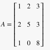
If we wanted to solve the system of equations shown above, we create a matrix containing the coefficients of the variables, which would be referred to as A in the equation Ax=b.

Now, we need to find the inverse of A.  We start by writing an Identity matrix to the left of the original matrix A. This is called an augmented matrix.

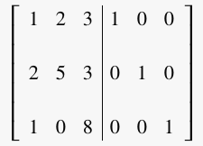
Note: The Identity matrix is equivalent to the number “1”.

1. It is square (has the same number of rows as columns)
2. It has 1s on its diagonal and 0s everywhere else
3. Its symbol is the capital letter I

Next, we must transform matrix A on the left into the Identity matrix.  The Identity matrix on the right just comes along for the ride. We transform the matrix by using elementary row operations.

Elementary row operations include:

1. Swapping rows
2. Replacing a row by adding or subtracting a multiple of another row
3. Multiplying and dividing each element in a row by a constant

These operations must be done to the whole row.  If a row of zeros results in the matrix on the left, then the original matrix A does not have an inverse.

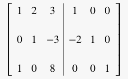
Step 1: Make zeros in column 1 except entry at row 1, column 1 (pivot entry)

Subtract row 1 multiplied by 2 from row 2 (R₂ = R₂  - (2)R₁):

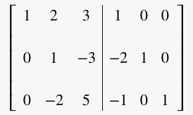
Subtract row 1 from row 3 (R₃ = R₃ – R₁ ):

Step 2: Make zeros in column 2 except entry at row 2, column 2 (pivot entry)

Subtract row 2 multiplied by 2 from row 1 (R₁ = R₁ – 2R₂ ):

Add row 2 multiplied by 2 to row 3 (R₃  =  R₃ + (2)R₂ ):

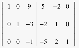
Step 3: Make zeros in column 3 except entry at row 3, column 3 (pivot entry):

Add row 3 multiplied by 9 to row 1 (R_{1 =} R₁ + (9)R₃):

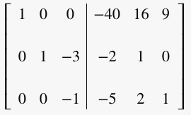
Subtract row 3 multiplied by 3 from row 2 (R₂ = R₂ – (3) R₃ ):

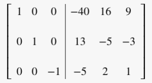
Multiply row 3 by -1 (R₃ = -1 · R₃ ):

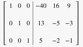
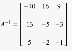
Now that we have the inverse of matrix A, we can solve for x by multiplying the inverse of A by the b vector which are the numbers (5,3,7) on the right of the equal sign from our equations above.

B =

x =

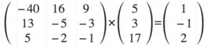
Therefore, the solution to the system of equations is (1,-1,2) which could represent the location of the cell which stores the desired metric we want to retrieve in our report.

So, the next time you’re pivoting data at a finger flick, take a moment to thank the ancients for their mathematical ingenuity. Without a doubt, we stand daily on the shoulders of giants.

Intricity Experts Article by:

Michael Fung