Algorithms That Run The World

An algorithm is a set of instructions to accomplish a task. There are literally thousands of algorithms that have had a huge influence on the world. Some have earned billions of dollars for their creators and their respective companies. The goal of this whitepaper is to highlight some of the algorithms that act as the heartbeat of the world that we occupy. Some of these are the unsung algorithms that are often the bedrock for other more well-known algorithms. But make no mistake, they represent the bedrock from which much of our modern conveniences are devised.

The secondary goal is to attempt to decrypt these algorithms into a form consumable to mere mortals, and provide reference to further deep dives, should there be interest.

Binary Enumeration 

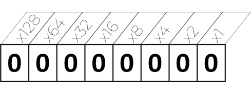
The bedrock of computing is the on/off switch. Everything you do on your computer, over the internet, on your phone, lives in binary. One of the superpowers in binary is the ability to enumerate absolutely unique values with a minimal amount of physically occupied space. Binary is a positional enumeration system with each digit in the registry representing a base multiple that doubles up as it scales. Here’s how the registry is laid out. Notice that each position is a power of 2. So as you progress up the scale, you’re increasing by that power 2⁰=1, 2¹=2, 2²=4, 2³=8, 2⁴=16….. For the representation below I’ve provided the exponential number written out. 

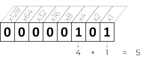
So the number 5 would be represented as:

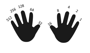
But the exciting part of binary numbers is the ability to represent very large numbers in a fixed space. For example, if you use your own hands, just your 10 fingers can count up to 1,023.

But consider the fact that a modern registry is operating at 128 positions! That’s 2¹²⁸ at the top registry number which in base 10 (normal notation) would be 340,282,366,920,938,463,463,374,607,431,768,211,456 or roughly 340 Undecillion, represented by only 128 registry positions! What this means is that there is a tremendous number of unique values that can be represented in a tiny space, which is what Binary Enumeration takes advantage of. 

By assigning numeric values to certain features you want to identify, those unique items can be flagged, allowing them to be referenced for computation in Binary operations. For example, in the early years of the telecommunications industry, customers used to be charged on a combination of tolls. There were tolls for international calls, tolls for regional calls, tolls for different offerings, etc. From call to call, those tolls could add up to formulate a specific bill. The sheer number of different tolls made binary enumeration a perfect way of building a unique identifier so they could be stacked up and added together after each call.

The same thing is done in modern video games that stack player attributes. 

Diffie-Helman Key Exchange

Our ability to communicate online without a million peering eyes is credited to Ralph Merkle, Whitfield Diffie, and Martin Hellman (with the latter two getting their names tagged to the exchange method).

Prior to Diffie-Helman, all the cryptography methods had one common drawback. They required a physical or agreed cipher, like the Nazi German Enigma machine which was used to decode messages and evaded the Allies until the advent of Alan Touring’s computer. 

So how do you share a secret between two parties without the presence of a pre-established decoder? Enter the Diffie-Helman Key Exchange. This exchange is done mathematically leveraging the power of binary enumeration registries to represent monstrous numbers, which makes the decryption very costly, if not impossible, to execute depending on the size. These numbers are exchanged in a form of private and public keys. The mixture of these keys decrypts the message. One way to visualize this exchange is by imagining the enormous numbers are colors of paint being exchanged.

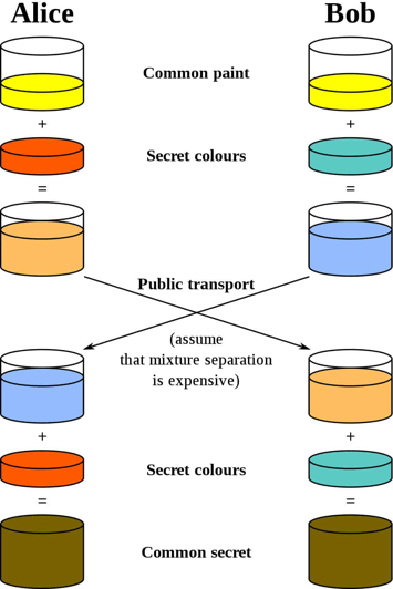The “Public Key” would be the common paint between Alice and Bob. This is a key that everybody can see. The common paint is mixed with a secret color then transferred over a public network. The sheer size of the numbers makes guessing the actual key much more difficult to accomplish, thus safe for public transportation over the web. When the message is received the recipients mix their secret colors in and the resulting color is a match decrypting the code. Of course, mathematically, the secret color of the recipient establishes a common secret between the two parties. Today there are many variants of this concept in practice that secure our communications. However, we still leverage the fundamentals of the Diffie-Helman Key Exchange for global communications.

Directed Acyclic Graphs

A Directed Acyclic Graph, or DAG, is so foundational that most people don’t even think of it as an algorithm. Yet its primal rule set is used in programming, mathematics, package shipping, network traffic, plumbing, electricity grids, oil pipelines, database queries, machine learning, and even processes within our own brains!

The basic concept of a DAG is a process that flows in a particular direction and does not loop. So let’s go over an example of something that isn’t a DAG and something that is, and we’ll do it within the same context.

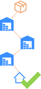Let’s say you buy an item on Amazon. The route your package will travel will follow a DAG with your house being the direction of the end state. The exact route the package might travel may vary between shipments, but one thing that should not happen is that the package goes back to one of the distribution points. If that does happen you know there’s a problem, and so does Amazon. So the shipping process at a package level is a DAG.

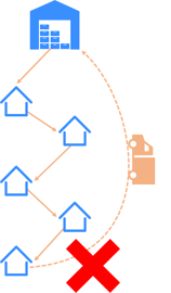However, the process that your local shipping truck follows is not a DAG. That might sound counterintuitive because the truck shouldn’t stop at a house twice, but ask yourself this. Once the route is done, could the driver leave the truck wherever his last stop was? No. The driver's process isn’t done until the truck returns to the distribution center. So if there are loops between the start and end of a defined process that process is not a DAG. So within the context of your specific package’s route, the shipping is a DAG, but the delivery truck’s end-to-end route is not.

If you would like to delve into the mathematics of DAGs, I would recommend a University of Cambridge publication which delves into “The Algebra of Directed Acyclic Graphs”. https://www.cl.cam.ac.uk/~mpf23/papers/Algebra/dags.pdf

TCP/IP

TCP/IP is the reason you can access the world from your computer. The system was created as part of a Department of Defense solution for accessing information over a limited bandwidth wire. The original standard was called a “4 layer model”. This layering was designed to make it possible to traverse the different carriers of data packets in order to serve up content to the right party. These four layers allowed the very complex task of directing data from Point A to Point B to be broken down into much more manageable steps.

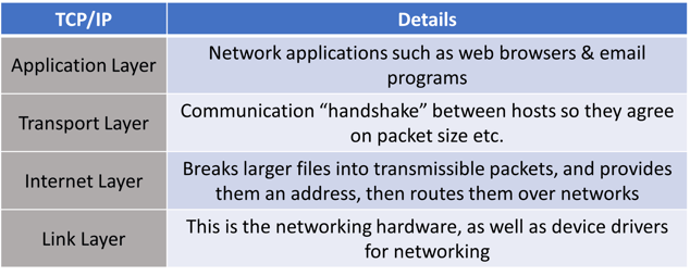As the TCP/IP matured into an agreed standard, it allowed different hardware manufacturers to transmit data to each other. A competing model called the OSI model which further broke down the TCP/IP gave TCP/IP a run for its money, but never was successful at unseating the standard. BUT network engineers used the layering concepts from OSI to further break down the TCP/IP standard. Here’s how they compare, with some sample protocols you might recognize:

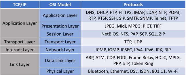
These extra layers give context to network engineers whether the issue they are dealing with is within their domain of control or not. 

Just as we spoke earlier about Binary Enumeration, networking uses this method to generate a unique enumeration of the IP location. This is done in a registry of 8 binary positions which in networking circles are called Octets. These octets are separated by a “.” and have 4 sets like this 192.168.0.1. The network reads this in binary, which would look like this, 11000000.10101000.00000000,00000001. If you refer back to the chart with the hand and you add up the first 8 finger positions it will add up to 255. So the maximum number for all 4 numeric positions is 255.255.255.255, or 11111111.11111111.11111111.11111111.

When you’re browsing the internet, you’re usually not directly connected to the hosting provider, rather you have a router that is managing all the broadcasting signals of the devices. The 4 octets we discussed earlier are made up of two parts, one that identifies the network which is called the network address, and the other that identifies the device which is called the host address. As the host broadcasts to the router, the router then broadcasts to the hosting service, and the hosting service broadcasts to the larger global network. This broadcast layering and how to route them is controlled by several proprietary protocols. However, some of the more well-known ones are the Distance Vector Routing Protocol and Link-State Routing Protocol.

Distance Vector Routing

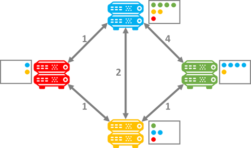
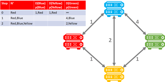
In Distance Vector Routing (DVR), each router shares data about how far its neighboring routers are. Each router has a table that keeps this information and it gets shared between adjacent routers. So imagine I have 4 routers that I switch on. What will happen in the beginning is that each router will share “distance” measures from the other. At the outset here’s what it might look like:

However, once each router finally propagates its router table, the fastest route can be determined by summarizing the distance as each share the routing tables between each other. The router at that point only needs to sort by the shortest route. So after the tables have been propagated the Red router will prioritize traffic to green through the Yellow router. The same will be true from Green to Red. Additionally, the Blue to Green will also prioritize the faster route through the Yellow router. Thus the prioritized router tables determine the shortest route based on the shortest adjacent distance to get to the end state:

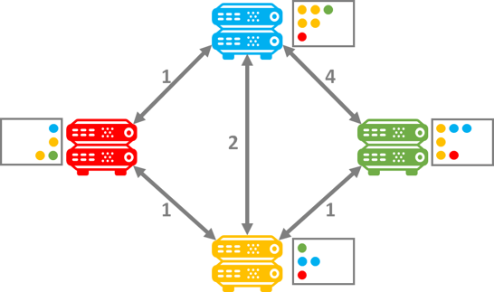
Notice how the Green router has changed its speed to the blue router from 4 to 3 once the router tables have propagated. If you would like to dive into the math of this algorithm, I suggest reviewing the GeeksforGeeks article on the topic: https://www.geeksforgeeks.org/distance-vector-routing-dvr-protocol/

The disadvantage of Distance Vector Routing is that it really doesn’t “know” anything about the actual network, just its closest neighbor, and a fairly crude metric on “distance”. This is where Link State Routing moved the torch further.

Link State Routing

Link State Routing is a lot more nuanced in its approach, and the shared data is much more extensive about the network. The routers start in a similar way, but instead of local nodes, the routers will first do a census of each other's adjacency by sending out a “hello” message. If the routers do determine they are adjacent they will share each other's Link State Advertisement or LSA. The LSA contains the router information, which connected links it has, and the state of those links. So rather than just hearing information about the adjacent neighbors, the LSA routers know about the entire adjacent network. That information is stored in a Link State Database on each router. 

Once this database is built, the fastest route is determined with a much more nuanced algorithm to determine the right route. This more nuanced routing is far more effective and intelligent. Updated information gets passed around to the different databases about every few minutes, so the network is always staying in sync. The power of this is that the network is aware of the actual linkages as a whole, and the databases can receive intermittent updates. The routing algorithms calculate a much more comprehensive evaluation of the fastest route than distance vector as it will actually survey the entire adjacent set of nodes and build a database table of results that are constantly being updated.

Each router sorts a calculated survey from each of its neighboring performances and stores it as a computed data set that sorts the results. There is an excellent course on the topic from Epic Networks Lab’s Youtube channel which outlines the Dijkstra link-state routing algorithm.

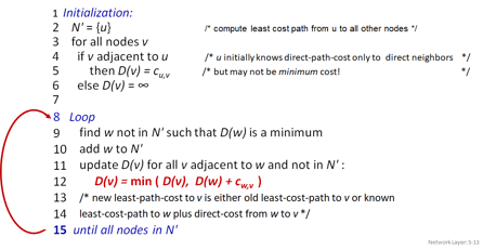
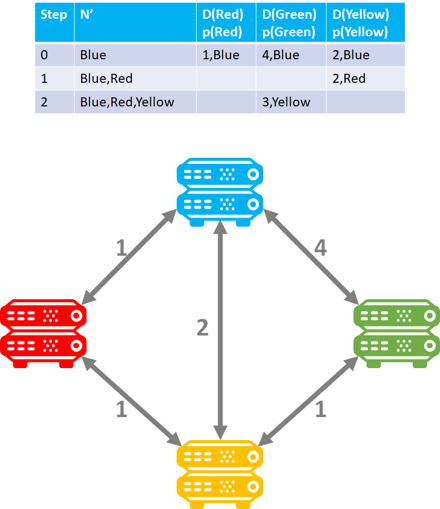
The notation and programming is as follows:

Doing this would render the following table for the Red router which would then sort the results for prioritization.

Here is an example of the Blue router:

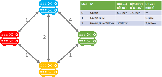
And the green router:

Database Optimizers

This last category really represents a host of algorithms, but with Intricity being so tied to data, it had to make the list. Most people think that they are speaking directly with enterprise databases when they write SQL queries. The reality is that they’re really speaking to an intermediary set of algorithms called a database optimizer which generates a query plan before the execution actually happens. Each vendor has a few interesting tricks up their sleeves based on their data architecture. 

The compilation of a query plan may be more about what is NOT queried than what is. Not only is it more efficient to exclude data from being scanned, but certain data may be sensitive in nature, and excluded therefore from the user. Query optimization often uses data partitions to determine whether a subsection of data should be scanned or not by persisting a min-max value on the partition of data. If the value fits within the min-max, it will scan the partition. Snowflake, for example, greatly expands this by automatically segmenting its partitions into 16MB chunks, which they call micro-partitions. When the database optimizer runs a query it quickly eliminates all the micro-partitions that are unrelated to the query by scanning the min/max values.

From that point, most database optimizers will use the smallest to biggest query route. This will usually involve some kind of anchor table that has the most succinct, clean, fast, data set that can be queried. For example, a sorted date table. The fastest way to optimize the query is to do a join on that clean anchor table, as the remaining scans will be constrained to smaller and smaller segments.

An additional important part of a query optimizer is the use of cache. If the query is a repeat, the optimizer’s algorithms will prioritize the cached version to provide an instant response.

The best Data Architects are the ones that study how to cater to the database optimizer’s strengths. For example, if queries are too dynamic then they will have a hard time being cached. If tables are loaded without sorting orders, the optimizer can have a hard time building an anchor set that can effectively daisy chain optimal queries.

If you would like to investigate more about optimizers, I recommend reading an article written by BrainKart.

Foundational, Yet Just a Handful

Here we’ve only listed 5 different categories of algorithms that are foundational to our way of life. They are used so regularly that at times we are unaware they represent the building blocks of much more complex processes. There are so many more amazing algorithms like BlockChain, PageRank, Backpropogation, Compression, and many others. All of these algorithms deserve a place in our minds, as these are some of the strings connected to our reality.